tl;dr Skip to the Summary.

In the appendix of 19-line Line-by-line Python Perceptron, I touched briefly on the idea of linear separability.

A perceptron is a classifier. You give it some inputs, and it spits out one of two possible outputs, or classes. Because it only outputs a 1 or a 0, we say that it focuses on binarily classified data.

A perceptron is more specifically a linear classification algorithm, because it uses a line to determine an input’s class. If we draw that line on a plot, we call that line a decision boundary.

I spent a lot of time wanting to plot this decision boundary so that I could visually, and algebraically, understand how a perceptron works. So today, we’ll look at the maths of taking a perceptron’s inputs, weights, and bias, and turning it into a line on a plot.

The first thing to consider is that a I’m only interested in plotting a decision boundary in a 2-D space, this means that our input vector must also be 2-dimensional, and each input in the vector can be represented as a point on a graph.

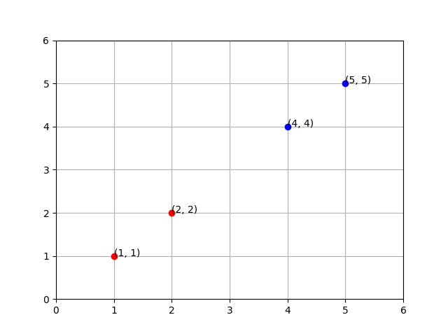
For example, the following training data can be plotted like the following:

x1 | x2 | label
----------------
1  |  1 |   0
2  |  2 |   0
4  |  4 |   1
5  |  5 |   1

Where x1 is the x and x2 is the y.

Once I’ve asked a perceptron to learn how to classify these labeled inputs, I get the following results:

weights:  [ 0.2, -0.1]
bias:  -0.29

And, when I ask it to classify an input that wasn’t in the training dataset, I get an intuitive result.

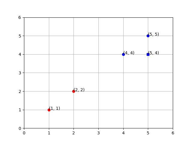
We can visually guess that the new input (5, 4) belongs in the same class as the other blue inputs, (though there are exceptions). We can also imagine the line that the perceptron might be drawing, but how can we plot that line?

Maths

Remember, the summation of that our perceptron uses to determine its output is the dot product of the inputs and weights vectors, plus the bias:

w · x + b

When our inputs and weights vectors of are of 2-dimensions, the long form of our dot product summation looks like this:

w1 * x1 + w2 * x2 + b

Since we’re consider x1 to be the x and x2 to be the y, we can rewrite it:

w1x + w2y + b

That now looks an awful lot like the standard equation of a line!

Ax + By - C = 0

Note: I’ve subtracted C from both sides to set the equation equal to 0.

We can now solve for two points on our graph: the x-intercept:

x = -(b - w2y) / w1if y == 0
x = -(b - w2 * 0) / w1x = -b / w1

And the y-intercept:

y = -(b - w1x) / w2if x == 0
y = -(b - w1 * 0) / w2y = -b / w2

With those two points, we can find the slope, m:

point_1 = (0, -b / w2)
point_2 = (-b / w1, 0)m = (y2 - y1) / (x2 - x1)m = (0 - -(b / w2)) / (-(b / w1) - 0)m = -(b / w2) / (b / w1)

Now, we have the two values we need to to construct our line in slope-intercept form:

slope = -(b / w2) / (b / w1)
y-intercept = -b / w2y = (-(b / w2) / (b / w1))x + (-b / w2)

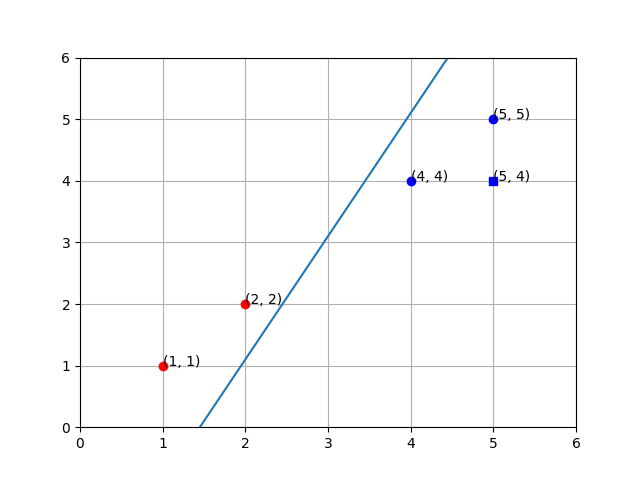
Plugging in our numbers from the dataset above, we get the following:

y = (-(-0.29 / -0.1) / (-0.29 / 0.2))x + (-(-0.29) / -0.1)y = (-2.9 / -1.45)x + -2.9y = 2x - 2.9

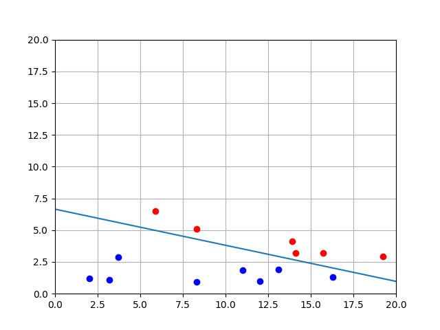
Plotting the Line

Summary

For a perceptron with a 2-dimensional input vector, plug in your weights and bias into the standard form equation of a line:

w1x + w2y + b = 0

Solve for the x- and y-intercepts in order to find two points on the line:

x_intercept = (0, -b / w2)
y_intercept = (-b / w1, 0)

Solve for the slope:

m = -(b / w2) / (b / w1)

Fill in the slope-intercept form equation:

y = (-(b / w2) / (b / w1))x + (-b / w2)

Resources

• https://brilliant.org/wiki/perceptron/
• Stack Overflow — How do you draw a line using the weight vector in a Linear Perceptron?
• Python Machine Learning — Part 1 : Implementing a Perceptron Algorithm in Python
• Standard form for linear equations - Khan Academy
• Tariq Rashid — A Gentle Introduction to Neural Networks and making your own with Python